Neural Turing Machines
These are, without a doubt, my favorite advancement in neural network technology. The goal of this blog is to elucidate the machinations of the Neural Turing Machine (NTM) and use a TensorFlow implementation to demonstrate some of the tasks that they’ve been trained to perform. Here’s the stuff I’m going to talk about:
- What they can do
- Architecture
- Math
- Implementation in TensorFlow
- Training tasks
- Oneshot learning
The NTM is demonstrably well-suited to performing memory-related tasks, such as: storing and recalling a sequence of bits, associative recall, and, to some extent, sorting data based on priority values (section 4). Additionally, further work has shown that vanilla NTM’s are quite capable of oneshot learning. Oneshot learning, also known as meta-learning, is a method of teaching neural networks how to learn (section 5).
1. What They Can Do
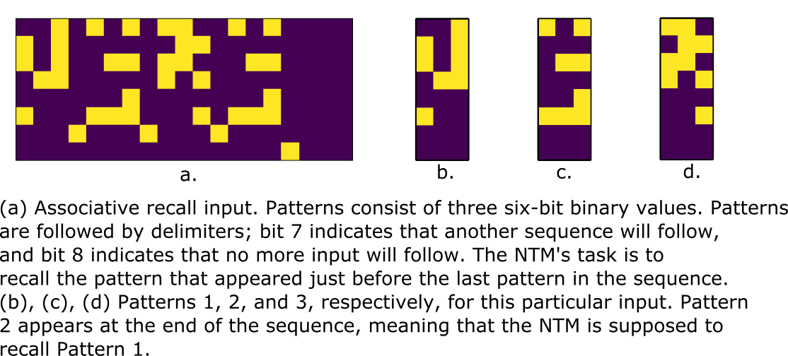
This is an example of one of the things that the NTM can do: associative recall. The task proceeds as follows:
- The NTM is presented with a series of random patterns [p1, p2, …, pn] with delimiters between each pattern
- The NTM is then presented with a pattern that was seen in the series of patterns, pi, followed by a special ‘stop’ delimiter
- The NTM is supposed to spit out the pattern that was seen immediately before this pattern, pi-1 (unless pi = pn, in which case the NTM would recall p1)
An example of the input is shown below:
This task is extremely difficult for RNN’s, even for deep Long Short-Term Memory (LSTM) networks, and in most cases they incur greater error as the number of patterns increases. But it’s a cinch for the NTM because it has the ability to perfectly store and recall information that it’s seen at all timesteps (though the size of the memory matrix is a limiting factor). The NTM can also produce a general solution when an arbitrary number of patterns are used, even if it was never explicitly trained to work with a given number of patterns. Other RNN architectures cannot generalize past what was seen in training.
2. Architecture
NTM’s technically fall under the category of recurrent neural networks (RNN’s). Traditional RNN’s store a representation of the data that’s been seen at previous timesteps. The NTM has the potential to store all data that from previous timesteps and perform operations explicitly on that data. This makes the NTM well-suited for learning small programs. The NTM works well with time-series data, and in most applications the NTM is presented with sequences of information, and then asked to perform some sort of operation (or operations) on that data, and that operation usually ends up being time-dependent.
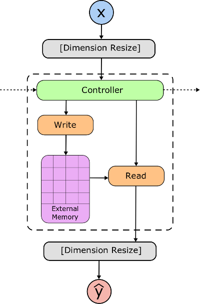
The NTM consists of four core components (see figure below). They all inter-rely on each other heavily, so it’s hard to talk about one component without talking about the others… but this organization seems to make sense:
- External memory matrix
- Controller network
- Read/write heads
External Memory Matrix
The memory matrix is literally just a repository of information that the controller saves. Data in the memory matrix is accessed (for reading or writing) by addressing a particular row of the matrix. The matrix is called ‘external’ because it isn’t trained through error backpropagation. An example memory matrix is shown below.
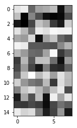
The matrix is 15x8, meaning that there are 15 memory addresses (rows) that can have 8 “bits” of information stored in each address. I have to use “bits” in quotation marks because the values are in the range [0, 1]. Analog bits…?
Controller Network
The controller’s job is to learn how to produce activations that read-from and write-to the memory matrix according to the process specified by the training data. In essence, the controller attempts to learn a program that allows it to use the read and write heads as advantageously as possible.
The controller network can consist of any combination of feedforward networks and RNN’s, but various experiments by the good people at Deep Mind have shown that an RNN controller produces the best results. The only restriction on the controller network is the number of outputs on the output layer; for every timestep in the task, the controller produces values that are used to read and write from the memory matrix.
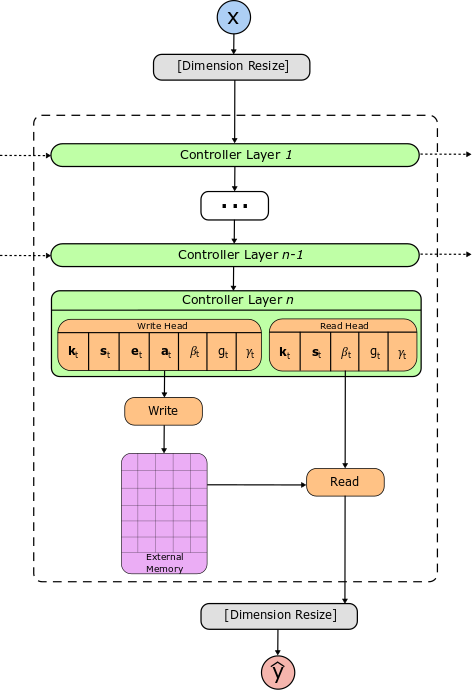
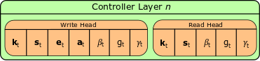
The boxes in green show the layers of the controller. The arrows entering/exiting the controller layers on the left/right sides show that the layers can possibly be RNN’s. The vector values emitted from the last layer of the controller network are used to write-to and read-from memory. Most importantly, the nodes/neurons on the last controller layer are split into pieces, and several different activation functions are applied to those pieces. The different activation functions allow us to control the range of values we get from the controller, and ultimately let us perform the reading and writing operations.
Read/Write Heads
Both the read and write heads consist of a soft attention mechanism that allow them to focus on parts of the memory matrix. What’s cool is that the read/write heads can also choose to focus on none of the values in memory. When you imagine a soft attention mechanism imagine a one-hot vector, or any vector with normalized elements (see below).
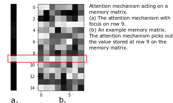
The row with the bright spot corresponds to the row of the memory matrix that we’re giving attention to.
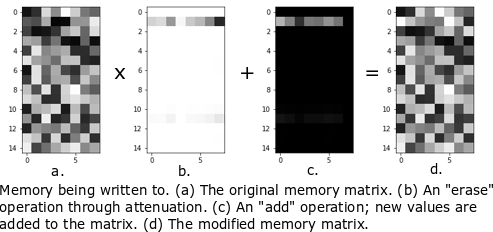
In addition to an attention mechanism, the write head produces erase and add vectors which remove data from memory and add data to memory, respectively. This can be used to overwrite or modify an existing entry, or add information to an unused memory location. An example of this is shown below (white pixels have values close to 1, black pixels close to 0).
The read and write heads can produce attention at different places in memory, which allows the NTM to write-to memory and read-from memory separately. In this implementation we force the NTM to write first and read second.
As an aside, the NTM can use multiple read/write heads, but we’re going to limit outselves to just one read/write head.
3. Math
All right, so where do the attention mechanisms come from? We said before that the read/write heads produce addresses to focus on different locations, but the math to create those addresses is exactly the same for both heads. The read/write heads produce a kt, st, βt, gt, and γt (see below). Note that emboldened variables represent vectors, capitalized variables are matrices, and lower-case, non-bolded variables are scalars.
| Piece | Name | Description | Activation |
|---|---|---|---|
| kt | Key | Emitted for content-based addressing. | None |
| βt | Key strength | Sharpens address generated from content-based addressing. | Softplus |
| gt | Gate | Interpolates between content-based address and address used at the previous timestep. | Sigmoid |
| st | Shift | Shifts the current address to a potentially different location. | Softmax |
| γt | Sharpen | Sharpens the result of the shift operation. | Oneplus (softplus + 1) |
| et | Erase | Removes data from the memory matrix. | Sigmoid |
| at | Add | Adds data to the memory matrix. | Sigmoid |
The first five variables are used to build addresses to access data from memory, and the last two are used to modify what’s stored in memory. Each variable has a time-subscript, meaning that the controller can emit brand new values for these variables at each timestep in the task. For now we’re only concerned with focusing on a particular memory address, which the NTM does by:
- generating an address based on data already in the matrix (content-based addressing)
- interpolating between the content-based address and the address used in the previous timestep
- shifting the address to a new location using circular convolution
- sharpening the result of the shifting operation.
In keeping with the original paper, we’ll call the final address wt, and all intermediate steps will be some superscripted version of wt. We’ll use parentheses notation to indicate that we’re accessing a particular element of a vector, e.g. w(i)t, and we assume that vectors are 0-indexed.
Content-Based Addressing
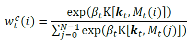
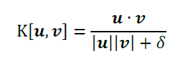
The goal of content-based addressing is to allow the NTM to create addresses based on items already in memory. Here we use the key, kt, and key strength, βt. The key is compared to each row of the memory matrix, Mt(i) using cosine similarity (the function K(.) shown below), and the result of this comparison is a vector. The similarity vector is multiplied by the key strength, βt ∈ [0, ∞), and the scaled similarity vector is passed through a softmax operation.
So what’s the importance of these things?
The key emitted by the controller network bears some degree of similarity to an element already in memory, meaning that the NTM can potentially group items in memory based on their similarity to each other. Note that the key could also be completely dissimilar to every memory element. The key strength serves two purposes: for βt » 1, the generated address becomes heavily sharpened around a single value; for βt < 1, the generated address becomes blurry, meaning that no particular content address is being focused on. When βt = 0 the content address becomes a uniform distribution over all possible memory addresses.
The cosine similarity calculation is probably something you’ve seen before. A small numerical value δ = 10-8 is added to the denominator to prevent loathsome 0/0 errors. Note: the address isn’t strictly a probability distribution, we don’t sample from the attention vector to obtain an address, but it is normalized such that all of the elements sum to 1.
Interpolation
At this point, the NTM uses gt ∈ [0, 1] to choose whether the content-based address or the address from the previous timestep, wt-1, has more effect on the final address, wt.
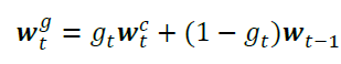
At this point the interpolated address wgt is still normalized, so we could just allow this to be the final address value. But this would be bad news if we wanted the NTM to be able to linearly scan through all of its memory addresses, so the NTM has two more steps that allow it to shift the interpolated address to a new location.
Shifting
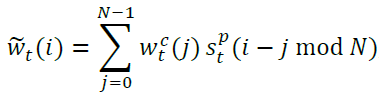
The NTM can take the interpolated address and shift its focus to a new address. It does this through circular convolution (you DSP folks will probably have seen this before). This step required the most troubleshooting in code, so I’m going to spend a bit of time on it, and I’m going to jump straight into the tricks that I used. The circular convolution equation is shown below.
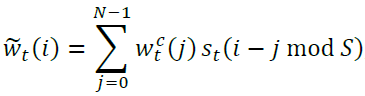
The shift vector, st has S elements where 2 ≤ S ≤ N (where N = the number of memory addresses). The vector is normalized, so all of the elements sum to 1. We get the address to shift by assigning mass to different indices of st. We also want our shift vector to be able to move the address forward or backward or not move the address at all.
First, we choose an index of st that corresponds to no movement, which we’ll call the center index. Then all indices to the left of the center index will move the address backward (decrement), and all indicies to the right will move the address forward (increment). The center index c is defined as the floor of S/2 (see below).
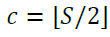
So an st with 5 elements would have index 2 at the center, etc. But just because we say that the elements to the right and left of the center should move the address, it doesn’t mean that they actually will. In order for this to work, the center index has to actually be at index 0, and the index that decrements the address by 1 should be at index N-1. But if we only have S < N elements in st, how can we possibly have any values at index N-1? Zero padding.
The next thing that we do is pad st with exactly N-S zeros in such a way that index c is relocated to index zero. We do that by performing the following operation:
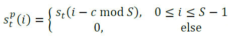
Ultimately we end up with a new shift vector, spt, with exactly N elements, which we use to perform the circular convolution.
The nice thing about zero-padding is that it keeps the vector normalized.
Sharpening
Convolution tends to “blur” things, so we offset this by exponentiating every term in the shifted vector and re-normalizing. Note that the exponentiation term is emitted by the controller, so the controller determines how much sharpening occurs.
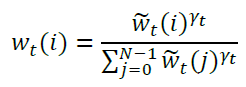
Note that γt is a scalar and is bounded as [1, ∞), so the worst that the controller could do is leave behind a blurry address. It’s interesting that the folks at DeepMind disallowed γt from being 0, which would allow the NTM to select all addresses with equal weighting (essentially performing a no-op).
4. Implementation in TensorFlow
Disclaimer: this implementation was created as part of a class project in the last year of my M.S. using TensorFlow v1.0.
The NTM is an RNN, and as such, we need to train it like an RNN. Luckily the TensorFlow (TF) API has an abstract class that allows us to define our own NTM class that can run and be trained just like any other RNN in the TF library. A slight downside to this is that we have to redefine the math in the previous section to work for matrices of input rather than vectors. Since the NTM operates on time-series data, training occurs over minibatches that are defined as rank-3 tensors. These tensors have a shape of [batch_size, sequence_length, vector_size], where
- batch_size is the number of training sequences being passed to the network
- sequence_length is the total number of timesteps, or the length of the training sequences
- vector_size is the size of an individual vector being passed to the network as input
As an example, let’s imagine that we’re training a language model with a 5000 word vocabulary with individual words represented as a one-hot encoding. At training time we want to give the network 64 sequences with 100 words per sequence (a sequence of words from a book or newspaper). This means that we’d pass the network a training tensor of size [64, 100, 5000].
I’m not going to get into the details of backpropagation through time, but there are a few things that need to be taken into consideration before we start coding. The NTM will receive slices of the training minibatch at each timestep. So for the first timestep, the NTM will receive a matrix of size (using our example above) [64, 5000] corresponding to the elements at [:, 0, :] from the original minibatch. At the next timstep, the NTM will receive another slice of the same size as the previous, this time corresponding to [:, 1, :]. As this happens, TF works its magic by computing gradients and updating our network’s weights.
Sizes of Relevant Vectors/Matrices
I’m adding this as a reference because we’ll need it when we implement the RNNCell class.
| Item | Size (number of elements) |
|---|---|
| Mt | N x M |
| kt | M |
| βt | 1 |
| gt | 1 |
| st | S |
| γt | 1 |
| et | M |
| at | M |
Note that all of these items only depend on three integers: N (the number of memory addresses), M (the representation of a particular element in memory), and S (the number of allowable address shifts made available to the controller).
The RNNCell Class
Let me elucidate exactly what our RNNCell class will be doing; our NTMCell will take the output of the controller (the various pieces from the very first table in the blog), use it to create read/write addresses, and perform read/write operations on the memory matrix. What’s interesting about this class is that it contains no trainable variables; all of the trainable variables will be contained solely in the controller network.
Ok, so there are a few methods that we’re required to implement, namely: __init__, state_size, output_size, and __call__. Let’s start with the __init__ method and work our way through the rest. Below is the entire listing, I’ll explicate the details of each method:
from __future__ import print_function

import collections
import math
import numpy as np

from tensorflow.python.framework import dtypes
from tensorflow.python.framework import ops
from tensorflow.python.ops import array_ops
from tensorflow.python.ops import clip_ops
from tensorflow.python.ops import embedding_ops
from tensorflow.python.ops import gen_math_ops
from tensorflow.python.ops import init_ops
from tensorflow.python.ops import linalg_ops
from tensorflow.python.ops import math_ops
from tensorflow.python.ops import nn_ops
from tensorflow.python.ops import partitioned_variables
from tensorflow.python.ops import random_ops
from tensorflow.python.ops import variable_scope as vs

from tensorflow.python.ops.rnn_cell_impl import _RNNCell as RNNCell

class NTMCell(RNNCell):

  def __init__(self, mem_size, shift_range=3):
    self.N, self.M = mem_size
    self.shift_range = shift_range
    self._num_units = self.M*self.N + 2*self.N

  @property
  def state_size(self):
    return self.N*(self.M,) + (self.N, self.N)

  @property
  def output_size(self):
    return self.M

  def __call__(self, inputs, state, scope=None):
    M = self.M
    N = self.N
    S = self.shift_range

    with vs.variable_scope(scope or 'ntm_cell'):
      mem_prev = array_ops.stack(state[0:-2], axis=1)

      w_read_prev = state[-2]
      w_write_prev = state[-1]

      write_pieces, read_pieces = self.head_pieces(inputs, (N, M), S)

      w_write = generate_address(write_pieces[0:5], w_write_prev,
        mem_prev, N, S)
      w_read = generate_address(read_pieces, w_read_prev,
        mem_prev, N, S)

      erase = array_ops.expand_dims(write_pieces[-1], axis=2)
      add = array_ops.expand_dims(write_pieces[-2], axis=2)

      w_write_ = array_ops.expand_dims(w_write, axis=2)

      erase_box = math_ops.matmul(
        w_write_, array_ops.transpose(erase, perm=[0, 2, 1]))
      add_box = math_ops.matmul(
        w_write_, array_ops.transpose(add, perm=[0, 2, 1]))

      mem_new = mem_prev*(1. - erase_box) + add_box

      read_w_ = array_ops.expand_dims(w_read, axis=1)

      reads = array_ops.squeeze(math_ops.matmul(read_w_, mem_new))
      state_tuple = tuple(array_ops.unstack(mem_new, axis=1)) + \
        (w_read, w_write)

    return reads, state_tuple

  def bias_state(self, batch_size):
    state_size = self.state_size
    start_bias = int(np.random.rand()*self.N/2.)

    bias_state = [
      np.abs(np.random.rand(batch_size, s))
      for s in state_size[0:-2]
    ]

    normal = np.zeros((batch_size, state_size[-1]))
    normal += 1./float(state_size[-1])
    one_hot = np.zeros((batch_size, state_size[-1]))
    one_hot[:,start_bias] = 1.
    #for i in range(batch_size):
    #   hot_index = int(np.random.rand()*self.N/2.)
    #   one_hot[i, hot_index] = 1.
    bias_state.append(normal.copy())
    bias_state.append(one_hot.copy())

    return tuple(bias_state)

  @staticmethod
  def head_pieces(head, mem_size, shift_range, axis=1, style='tuple'):
    N, M = mem_size
    S = shift_range
    center = int(S/2.)
    shift_bias = np.zeros(S)
    shift_bias[center+1] = 2.5
    #print(write_head_raw.get_shape(), read_head_raw.get_shape())

    # Fix the stupid head splitting; you changed it so that you wouldn't
    # have to concatenate/split crap inside of ntmagain.py

    # Number of elements in the read/write heads, respectively.
    splits = [M+S+3, 3*M+S+3]
    read_head_raw, write_head_raw = array_ops.split(head, splits,
      axis=axis)

    write_pieces = array_ops.split(write_head_raw,
      [M, S, 1, 1, 1, M, M], axis=axis)
    read_pieces = array_ops.split(read_head_raw, [M, S, 1, 1, 1],
      axis=axis)

    key_w, shift_w, gamma_w, beta_w, g_w, add_w, erase_w = write_pieces

    # Multiple operations are applied to the pieces of the write head,
    # see the original paper or this project's writeup for the breakdown.
    shift_w = nn_ops.softmax(shift_w + shift_bias)
    gamma_w = gen_math_ops.minimum(nn_ops.softplus(gamma_w) + 1, 21.)
    beta_w = nn_ops.softplus(beta_w)
    g_w = math_ops.sigmoid(g_w)
    add_w = math_ops.sigmoid(add_w)
    erase_w = math_ops.sigmoid(erase_w)

    key_r, shift_r, gamma_r, beta_r, g_r = read_pieces

    # Operations applied to the pieces of the read head.
    shift_r = nn_ops.softmax(shift_r + shift_bias)
    gamma_r = gen_math_ops.minimum(nn_ops.softplus(gamma_r) + 1, 21.)
    beta_r = nn_ops.softplus(beta_r)
    g_r = math_ops.sigmoid(g_r)

    if style=='tuple':
      write_head = (key_w, shift_w, gamma_w, beta_w, g_w,
        add_w, erase_w)
      read_head = (key_r, shift_r, gamma_r, beta_r, g_r)
    else:
      write_head = \
      {
        'key' : key_w,
        'shift' : shift_w,
        'gamma' : gamma_w,
        'beta' : beta_w,
        'g' : g_w,
        'add' : add_w,
        'erase' : erase_w,
      }

      read_head = \
      {
        'key' : key_r,
        'shift' : shift_r,
        'gamma' : gamma_r,
        'beta' : beta_r,
        'g' : g_r,
      }

    return write_head, read_head

def cosine_similarity(a, b):
  dot = math_ops.reduce_sum(a*b, axis=1)

  norm_a = linalg_ops.norm(a, ord=2, axis=1)
  norm_b = linalg_ops.norm(b, ord=2, axis=1)

  # Some padding is added to the denominator to prevent 0/0 errors.
  cos_sim = math_ops.divide(dot, math_ops.add(norm_a*norm_b, 1e-8))

  return cos_sim

def circular_convolution(shift, w_i, N, S, zero_pad=False):
  zeros = array_ops.zeros_like(shift)

  split_loc = N % S
  center = int(S/2)
  #print('center:', center)
  #center = 1

  if not zero_pad:
      num_tiles = max(int(N/S), 0)
      if num_tiles > 0:
        shift_tile = array_ops.tile(shift, [1, num_tiles])
      else:
        shift_tile = shift

      if split_loc > 0:
        tack = array_ops.split(shift, [split_loc, -1], axis=1)[0]
        shift_long = array_ops.concat([shift_tile, tack], axis=1)

  else:
      num_tiles = max(int((N - S)/S), 0)
      if num_tiles > 0:
        zeros_tile = array_ops.tile(zeros, [1, num_tiles])
      else:
        zeros_tile = zeros

      if split_loc > 0:
        tack = array_ops.split(zeros, [split_loc, -1], axis=1)[0]
        shift_long = array_ops.concat([shift, zeros_tile, tack], axis=1)

  center_split = array_ops.split(shift_long, [center, -1], axis=1)
  shift_rev_ = array_ops.concat([center_split[1], center_split[0]], axis=1)
  shift_rev = array_ops.reverse(shift_rev_, axis=[1])

  circ = []
  for j in range(N):
    loc = (j + 1) % N
    shift_split = array_ops.split(shift_rev, [N-loc, loc], axis=1)
    circ.append(array_ops.concat([shift_split[1], shift_split[0]], axis=1))

  w_conv = [math_ops.reduce_sum(w_i*c, axis=1) for c in circ]

  return array_ops.stack(w_conv, axis=1)

def generate_address(pieces, w_prev, mem_prev, N, S):
  key, shift, gamma, beta, g = pieces

  w_c_arg = [cosine_similarity(m, key) \
      for m in array_ops.unstack(mem_prev, axis=1)]

  w_c_arg = array_ops.stack(w_c_arg, axis=1)

  w_c = nn_ops.softmax(beta*w_c_arg)

  w_i = g*w_c + (1. - g)*w_prev

  w_conv = circular_convolution(shift, w_i, N, S, True)

  w_sharp = math_ops.pow(w_conv, gamma)

  w = w_sharp/math_ops.reduce_sum(w_sharp, axis=1, keep_dims=True)

  return w
If you look at the definitions of other classes that inherit from RNNCell, you’ll see that they use the initializer to internalize some information about the cell being implemented (the number of units being used, types of activation functions, etc.). We already know what activation functions we’ll be using, all that we have to provide are values for N, M, and S.
def __init__(self, mem_size, shift_range=3):
  self.N, self.M = mem_size
  self.S = shift_range
We give the shift_range a default value of 3 because it works reasonably well for the experiments replicated from the paper. For the sake of clarity, having a shift range of three allows us to shift the address forward (increment its position), backward (decrement its position), or leave the address in the same location.
Pretty painless so far, now let’s implement the state_size method.
The RNNCell’s state size is the size of recurrent state that’s modified from timestep to timestep. Our hidden state will consist of the read and write addresses from the previous time step, as well as the memory matrix from the previous timestep. Our recurrent state will be a tuple containing (memory_row_1, memory_row_2, ..., memory_row_N, read_address, write_address). From the documentation we know that the state size can be a tuple of integers. Our state_size method looks like this:
def state_size(self):
  return self.N*(self.M,)  + (self.N, self.N)
So our recurrent state will be a tuple that contains each row of the memory matrix (in order), with the previous read and write addresses at the end of the tuple.
Still relatively painless, now on to output_size.
Our output_size is the size of the vector that’s regurgitated from the NTMCell. We’re going to use the output of the read head as the output of our NTMCell, which means that the NTMCell will have an output size of M (because the value that we read from memory will have eight elements in it). We don’t need to use a tuple here because we’re returning a single value.
def output_size(self):
  return self.M
The __call__ method is where the magic will happen. It takes in a batch of inputs and current states, and returns a batch of outputs and new states. The fact that it returns batches rather than vectors is important to us because it increases the rank of the tensors we return by one (note that a vector is a rank-1 tensor, matrix is a rank-2 tensor).
The interesting result of this is that our memory matrix, once assembled, will be a rank-3 tensor of size (batch_size, N, M).
Below is the code that’s used in the __call__ method to generate read/write addresses, read and write from memory, and update the recurrent state of the NTMCell.
def __call__(self, inputs, state, scope=None):

  M = self.M
  N = self.N
  S = self.shift_range

  with vs.variable_scope(scope or 'ntm_cell'):
    mem_prev = array_ops.stack(state[0:-2], axis=1)
    w_read_prev = state[-2]
    w_write_prev = state[-1]

    write_pieces, read_pieces = self.head_pieces(inputs, (N, M), S)

    w_write = generate_address(write_pieces[0:5], w_write_prev,
        mem_prev, N, S)
    w_read = generate_address(read_pieces, w_read_prev,
        mem_prev, N, S)

    erase = array_ops.expand_dims(write_pieces[-1], axis=2)
    add = array_ops.expand_dims(write_pieces[-2], axis=2)
    w_write_ = array_ops.expand_dims(w_write, axis=2)

    erase_box = math_ops.matmul(
        w_write_, array_ops.transpose(erase, perm=[0, 2, 1]))
    add_box = math_ops.matmul(
        w_write_, array_ops.transpose(add, perm=[0, 2, 1]))
    mem_new = mem_prev*(1. - erase_box) + add_box

    read_w_ = array_ops.expand_dims(w_read, axis=1)

    reads = array_ops.squeeze(math_ops.matmul(read_w_, mem_new))
    state_tuple = tuple(array_ops.unstack(mem_new, axis=1)) + \
        (w_read, w_write)

return reads, state_tuple
Most of the math is squirreled away behind functions, and that’s totally by design (the fact that these functions aren’t class methods is also by design; makes it easier to troubleshoot). The first lines 1-11 of the __call__ method are fairly self-explanatory, the line write_pieces, read_pieces = self.head_pieces(inputs, (N, M), S) simply splits the various vectors (kt, st, etc.) from the controller output and returns the sets of pieces from the read head and write head as a pair of tuples.